Modelling, Design and Validation of a Parallel Kinematic Robot for Additive Manufacture Applications

The additive manufacture is a fabrication process that has taken huge steps in the last decade, even though the first researches and prototypes are around since almost forty years ago. In this article, a design method for a Parallel Kinematics Robot for Additive Manufacturing Applications is proposed. A numerical model is obtained from the kinematics of the robot for which the design, construction and assembly are planned using recycled materials and equipment. The control of the robot is done using open source software, allowing the planning of trajectories in the Cartesian space on a maximum designed cylindrical workspace of 300mm in diameter by 300mm high. At the end of the work the robot was identified, the kinematic model was validated and considerations for future works were given.

Introduction

As of today there are many industries that use robots to increase their productivity. The manufacturing industry, that is in charge of transforming raw materials into finished products [1] is no stranger to automation. In fact, since the introduction of CAD (Computer Aided Design) and CAM (Computer Aided Manufacturing), the manufacture of products has become faster, more reliable, more precise and simpler [2] than before. Among the machines that work with CAD/CAM there are the CNC (Computer Numerical Control) machines and most of them work using material removal processes. Recently, however, these industries have been incorporating CNC machines for additive manufacturing processes.

Additive manufacturing, also known as 3D printing, has become very important in recent years. Not only allowing the production of prototypes or even finished products in shortest periods of time. But, also reducing the economic costs of prototypes compared to classic manufacturing processes by material removal or plastic injection [3]. This kind of technology outperforms when the production quantities are small or the products are customised. Moreover, compared to material removal manufacturing, additive manufacturing generates less material loss. Some authors estimate that up to 75% of the part costs are affected by damage done to the workpiece by the process [4].

Although additive deposition modelling has more than three decades since its invention as we know it today, it is not until the last ten years that thanks to the release of patents and advances in control, electronics and the benefits and facilities of computing in the field of CAD/CAM, a major breakthrough has been achieved in the reproduction of 3D printers [5,6]. Technological advances that bring at the same time a decrease in their costs. In a market where today for many companies from advertising and marketing agencies to large corporations and universities dedicated to architecture, design and engineering the use of 3D printers is indispensable.

For 3D printing devices, serial kinematic robots (or Cartesian robots) are commonly used. Their main advantage is the simplicity of construction and control. Although the drives must withstand the load of the subsequent links, so that both the speeds and accelerations are reduced due to the inertia of the system and the accumulated errors are greater in comparison with their parallel counterpart [7]. However, robots with parallel kinematics are being build for this kind of application. Although the construction and control of the parallel robot are more complex compared to serial architectures. Highest speeds can be achieved due to the kinematics and the reduced inertia of the parallel machine [7].

In this work, the objective is to determine the design of a robot with parallel kinematic chains with low inertia and high speeds for additive manufacturing applications. Obtaining a design methodology from the kinematic model, building the robot and validating the model from measurements on a real device. Thus, in order to achieve this, the manuscript is presented in six subsequent sections: ”State-of-the-art” reporting a literature overview for parallel kinematic mechanism for additive manufacture; ”Methodology” describing the methodology employed for the design studying the kinematics of the mechanism; ”Design” explaining some of the decisions made and limitations of the physical robot and presents the final design; ”Results” presenting the obtained results from the methodology; ”Discussion” analyzing the results and ”Conclusion” finishing the work and including a future works subsection in order to keep adding innovative developments in the field of parallel kinematic machines for additive manufacture.

State of the art

According to Schey (2002) [8], the manufacture is defined as ”the fabrication of goods and articles by hand, or especially by machinery, often on a large scale and with division of labor”. Kalpakjian (2002) [9] in the other hand states that the manufacture is the process of converting raw materials into products and includes:

1. The design of the product

2. The selection of the raw material

3. The sequence of processes through which the product will be manufactured.

Additive manufacture

In 2011, Cotec [10] mentions that what we know as Additive Manufacturing is basically the process of manipulating material on a small scale, layer by layer in a very precise way in order to create a built solid piece.

Additive fabrication can be classified depending on the process they use. Singh, et al. [11] identified seven different techniques: (1) Laser Melting, (2) Laser polymerization, (3) Extrusion Thermal, (4) Material Jetting, (5) Material Adhesion and (6) Electron Beam. Among these techniques, maybe the most popular is the Extrusion Thermal. The Extrusion Thermal has earned a lot of applications since its massive open-source availability. Communities like RepRap [6] has made 3D printing very accessible to all kind of users. Extrusion Thermal consists in the production of a part by the ejection of a thermoplastic through a nozzle, which runs typically thanks to a Cartesian mechanism through all the positions where material must be present, thus layer by layer the desired solid is shaped.

Nonetheless, not all 3D printers are mounted on serial kinematic mechanisms. It is possible to find 3D printers that thanks to the higher velocities, stiffness and precision advantages of parallel kinematic machines over their serial counterpart become a good choice for the manufacturing task.

Parallel kinematic mechanisms for additive manufacture

Parallel kinematic mechanisms or parallel robots are those which kinematic architecture contains one or more kinematic closed loops. According to Merlet [7], a parallel robot consists of a fixed base and an end-effector with n degrees of freedom connected by at least two independent kinematic chains, actuated by n single actuators.

Among the parallel robot with possible applications in the manufacturing industry one of the most interesting ones is the one presented by Seward et al. [12] in 2014, the Hexapteron, a novel six-chain parallel robot. The new six-degree-of-freedom robot is an extension of the Cartesian parallel robot. It consists of 3 pairs of prismatic actuators placed on the base, where the direction of each pair are the axes of the Cartesian coordinate system. In each of the chains there are two passive joints parallel to the direction of the prismatic joint. Concordly, these chains are coupled to the moving platform via universal joints. The direct kinematics can be easily solved by starting from the orientation and position of the platform. There are eight different solutions that are found directly by solving a linear system and alternating the signs of the three radicals. This robot has a large workspace and is suitable for machining or rapid prototyping applications. The Hexapteron is also a part of a family of robots called multipteron, starting from the tripteron [13], quadrupteron [14] and pentapteron [15] (of 3, 4 and 5 degrees of freedom respectively and are developed mainly by X. Kong and C. M. Gosselin).

Additionally, Stepanenko in 2016 [16] presented a 5 degrees of freedom parallel robot. This robot was based on 4 prismatic actuators capable of controlling all the three translations and one rotation of the platform of the robot. While, the fifth degree of freedom consisted in controlling the rotation of a working table of the robot. However, this machine can find use for future additive manufacture applications while at the moment can be a good candidate for machining applications.

Proceeding now with parallel robots and architectures that had already been applied in additive manufacture, in 2009 Briones [17] designed and analysed a parallel robot with 3 degrees of freedom consisting of two 5-bar mechanisms connected by two prismatic joints, with the robot platform at the junction of these two joints. He performed the calculation of the direct and inverse geometry, the jacobian matrix and the workspace from the methodology of analysis of serial and parallel mechanisms developed by Gogu (2008) [18]. Arriving to a detailed design and construction of the prototype.

Then in 2012, Hodgins, et al. [19] proposes an innovative design for the delta robot, increasing the useful workspace and reducing singularities. The inverse geometry, jacobian and stiffness of the robot are formulated and then used to calculate the different workspaces to illustrate the advantages of the new design. It then solves the optimisation problem and proceeds to make a 3D model of the model for subsequent construction and verification of functionality.

Later in 2013, Xuan Song, et al. [20] proposed the design and construction of a prototype of a six-degree-offreedom parallel robot based on the Stewart mechanism for low-cost additive manufacturing that can work on inclined planes. The project starts from the design of the robot, the cost of materials, the planning of movements and design of the control software, calibration of the platform and experimental tests from which a working space of 300mm x 300mm x150mm was obtained, an accuracy of less than 0.5mm when the direction of the tool is kept the same and that the angle of rotation of the platform is ± 30°. For future work they plan to improve the accuracy of the prototype system with better software and hardware and better calibration. In addition to testing for applications such as repair and construction around inserts.

In 2014, Amig`o [21], describes the development of a delta 3D printer, including the design of each part up to the construction of the machine. Obtaining a 3D printer for domestic use, with good results and low manufacturing costs, with the only drawback being a loss of precision due to the Bowden system of the extruder.

Methodology

The proposed prototype model is based on a philosophy of operational reliability as it is the first prototype of parallel kinematic robots for additive manufacturing designed and built from scratch as well as the first registered for academic purposes in Venezuela so far. Considering as a crucial factor the unavailability to state-of-theart workshops and supplies, the decision making around the design of the robot, as well as the design of some mechanical components is kept as simple as possible.

The whole robot was inspired by the modular design so that the project could at some point give life not only to a specific parallel robot but to multiple desired configurations reducing the chances of failure of the project. It was also designed under the premise of dimensional flexibility as a prototype for didactic and research purposes, with high possibilities of inaccuracy both from manufacturing and recycled equipment (adding an ecological point of view). The economic conditions of the project and available resources lead to recycling and reusing spare components from other machines.

For the design of the robot according to available resources and the previously considerations stated, we decided to develop a 3 degrees of freedom parallel robot composed by 3 kinematic closed loops based on an actuated prismatic joint and two subsequent universal joints. Then, the methodology proposed for this work is to first study the geometry of the mechanism. Starting from the study of the mobility of the robot, arrange of the robot base, geometry constraints and simplifications followed by the computation of the Inverse Geometric Model and Forward Geometric Model. Once we are done with the geometry we study the First Order Kinematics in order to identify the limits of the workspace i.e. the singularities of the robot. Up to this point we will limit the design of the robot but we will proceed with the experimentation after the assembly using open source software [6] to control the robot.

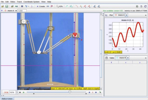
Afterwards, the experimentation part of this article is based on the evaluation and validation of the kinematics of the prototype. A helical trajectory will be executed on the prototype looking to have a wide range of motions of the joints. Following the motions, a visual tracker software [22] as shown in Figure 1 will be used in order to obtain measurements of the joint positions. Finally, from the analysis of the data we will proceed to conclude the work.

Modelling

Before proceeding with the simulation of the parallel robot, it is necessary to justify the choice of the type of parallel machine to be built. It was decided that the best choice for the robot is a linear delta type, as it is the most popular type for additive manufacturing applications and has enough online documentation that can facilitate the development of the work [6,17,21].

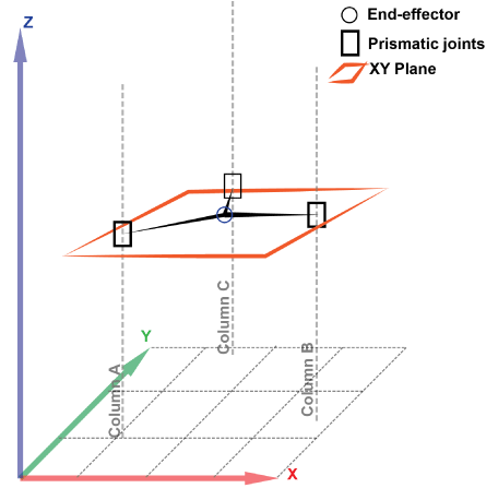
The linear delta robot is configured with three columns, three prismatic joints, six links and a platform where the end-effector is located. To determine the design, it is first necessary to carry out a kinematic study of the robot and to find its workspace defined by the jacobian matrix. Once it has been obtained, its singularity points are found and the robot is designed in such a way to avoid any possible singularity.

The ”Chebyshev-Grubler-Kutzbach” (CGK) [23] formula in equation (1) is then used to check the mobility of the mechanism and that the selected robot has three degrees of freedom as desired. This equation consists in a first part containing all the degrees of freedom of the rigid bodies and a second containing the constrained degrees of freedom from the joints of the whole mechanism. Where M is the mobility of the robot or the degrees of freedom, N represents the number of rigid bodies in the mechanism (counting ground), 5j1, 4j2 and 3j3 consists in the constrained degrees of freedom of the mechanism according to the total number of joints of one, two and three degrees of freedom that are present in the mechanism.

$M\mathrm{<mo>=</mo>6<mo\; stretchy="false">(</mo>}N-\mathrm{1<mo\; stretchy="false">)</mo>}-5j_1-4j_2-3j_3$ (1)

The number of rigid bodies present in our mechanism are 1 fixed base, 1 platform and for each of the 3 kinematic chains there are 1 slider link and 2 rod links for a total of N=11 rigid bodies. Regarding the joints, there are 1 actuated joint of one degree of freedom (j1) and 4 passive joints of 2 degrees of freedom (j2) for each of the 3 kinematic chains for a total of j1=3 and j2 = 12. Then, going back to equation (1) with N =11, j1=3 and j2 = 12 we compute the mobility M of the mechanism.

$M\mathrm{<mo>=</mo>}\mathrm{6<mo\; stretchy="false">(</mo>}N-\mathrm{1<mo\; stretchy="false">)</mo>}-5j_1-4j_2-3j_3$ $M\mathrm{<mo>=</mo>}\mathrm{6<mo\; stretchy="false">(</mo>3<mo\; stretchy="false">(</mo>1}+2+\mathrm{1<mo\; stretchy="false">)</mo>}-\mathrm{1<mo\; stretchy="false">)</mo>}-\mathrm{5<mo\; stretchy="false">(</mo>3<mo\; stretchy="false">)</mo>}-\mathrm{4<mo\; stretchy="false">(</mo>12<mo\; stretchy="false">)</mo>}-\mathrm{3<mo\; stretchy="false">(</mo>0<mo\; stretchy="false">)</mo>}$ $M\mathrm{<mo>=</mo>}\mathrm{6<mo\; stretchy="false">(</mo>11<mo\; stretchy="false">)</mo>}-\mathrm{5<mo\; stretchy="false">(</mo>3<mo\; stretchy="false">)</mo>}-\mathrm{4<mo\; stretchy="false">(</mo>12<mo\; stretchy="false">)</mo>}$ $M\mathrm{<mo>=</mo>}66-63$ $M\mathrm{<mo>=</mo>}3$

In this way it is verified that the mechanism does indeed have 3 degrees of freedom.

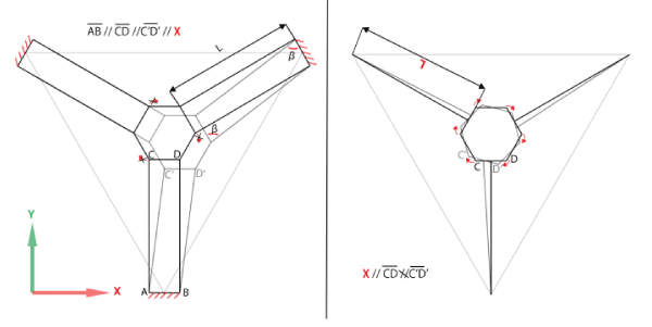
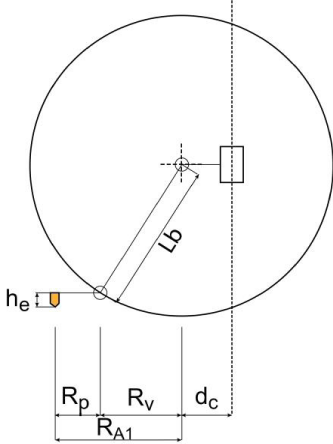
Before starting with the explanation of the kinematic model, we will simplify the 3 parallelograms to only 3 links instead of six, as six are used to constraint the rotational degrees of freedom of the platform as it can be seen in Figure 2. Additionally for the design, we took into account that in order to avoid the degeneracy of the parallelogram into a line one can use the same approach used by Coralie, et al. [24] and Briot, et al. [24]. Their approach consisted in constraining the workspace of the robot and setting a range of admissible values of the internal angles (Ø)of the parallelograms in order to prevent it to fall into singularity and degeneracy. For our design, we considered the range of angles used by Coralie, et al. [26], so the angle Ø was set to be between π/6 and 5π/6 to avoid any degeneracy problem of the parallelogram. The distances between the centers of the universal joints are considered in the length of the links. The link end shared with the carriage is named A1 while the one shared with the platform, A2. The diameter formed by the ends A1 of the links is called Diameter A1 (DA1) and in addition to this is the Virtual Radius term (Rv), which is obtained by subtracting the Diameter of the Platform (DA1)from the Diameter A1(DA1).

The model then is simplified as shown in Figure 3 by removing the distances that are constant in the robot such as (i) the distance of the joint A1 to the column axis, (ii) the platform radius Rp and (iii) the height of the extruder he.

$R_v\mathrm{<mo>=</mo>}\frac{D_{A_1}-D_p}{2}$

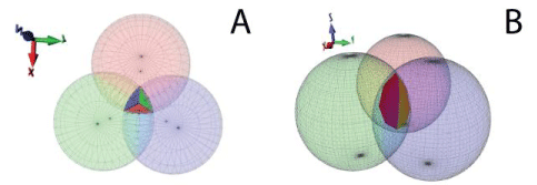
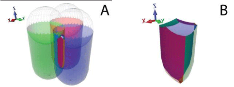
Thanks to the Virtual Radius, it is possible to simplify the behaviour of each kinematic chain as a sphere with a radius equal to the length of the links and with centers fixed in the XY plane with variable Z coordinate as depicted in Figure 4. The intersection of these spheres is the common point of the three links.

$x_i\mathrm{<mo>=</mo>}{R}_v\cos {\theta }_i$ $y_i\mathrm{<mo>=</mo>}{R}_v\sin {\theta }_i$ $z_i\mathrm{<mo>=</mo>}{d}_i$ ${\theta }_i\mathrm{<mo>=</mo>}\frac{\mathrm{<mo\; stretchy="false">(</mo>}i-\mathrm{1<mo\; stretchy="false">)</mo>2}\pi }{3}$ $i\mathrm{<mo>=</mo>1,2,3}$

Where Rv is the virtual radius of the mechanism, xi and yi are the centers of each sphere in the XY plane and di the joint position of the kinematic chain.

${\mathrm{<mo\; stretchy="false">(</mo>}x-x_i\mathrm{<mo\; stretchy="false">)</mo>}}^2+{\mathrm{<mo\; stretchy="false">(</mo>}y-y_i\mathrm{<mo\; stretchy="false">)</mo>}}^2+{\mathrm{<mo\; stretchy="false">(</mo>}z-d_i\mathrm{<mo\; stretchy="false">)</mo>}}^2\mathrm{<mo>=</mo>}{L}_b^2$ (2)

Inverse geometric model

Unlike serial kinematic robots, the inverse geometric model is obtained quite simply. To compute analytically the inverse geometry it is enough to isolate di from the canonical equation of the three spheres, thus obtaining:

$d_i\mathrm{<mo>=</mo>}z\pm \sqrt{L_b^2-{\mathrm{<mo\; stretchy="false">(</mo>}x-x_i\mathrm{<mo\; stretchy="false">)</mo>}}^2-{\mathrm{<mo\; stretchy="false">(</mo>}y-y_i\mathrm{<mo\; stretchy="false">)</mo>}}^2}$ (3)

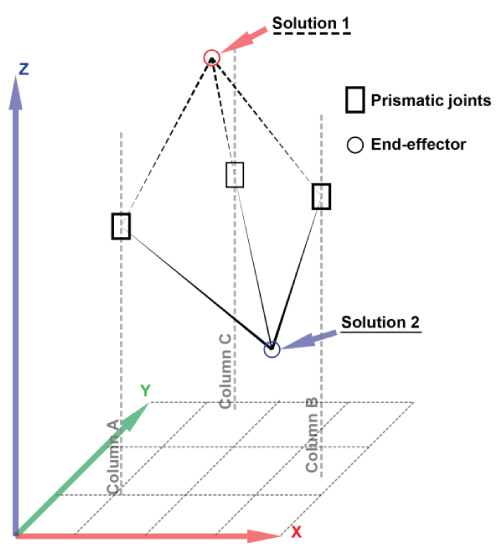
In the case of the present article we take from the equation (3) only one solution, i.e. the negative radical one as it can be seen in Figure 5. Thus obtaining a graphical representation of the workspace of the robot as depicted in Figure 6 and obtaining the function that enables us to compute the end-effector position related to that of the three prismatic joints.

Forward geometric model

Oppositely to the inverse geometric model, the deduction of the forward geometric model for a parallel robot is more difficult compared to that of a serial robot.

To find this model it is first necessary to make the intersection of a sphere with the others resulting in two planes, from these planes two straight lines x as a function z and y as a function of z are obtained. Subsequently, the variables x and y are substituted in one of the spheres to obtain a second degree polynomial equation whose unknown is z. In the same way as in the inverse geometric model, only the smallest result will be of interest and finally, from this, the results for x and y are obtained. The procedure is explained in detail below:

Firstly, we develop the square terms in each of the three canonical equations of the spheres, obtaining the next three equations:

$x^2-2x{x}_1+x_1^2+y^2-2y{y}_1+y_1^2+z^2-2z{d}_1+d_1^2\mathrm{<mo>=</mo>}{L}_b^2$ (4)

$x^2-2x{x}_2+x_2^2+y^2-2y{y}_2+y_2^2+z^2-2z{d}_2+d_2^2\mathrm{<mo>=</mo>}{L}_b^2$ (5)

$x^2-2x{x}_3+x_3^2+y^2-2y{y}_3+y_3^2+z^2-2z{d}_3+d_3^2\mathrm{<mo>=</mo>}{L}_b^2$ (6)

Subtracting equation (5) and (6) from equation (4) gives the equations (7) and (8) respectively:

$2x\mathrm{<mo\; stretchy="false">(</mo>}{x}_2-x_1\mathrm{<mo\; stretchy="false">)</mo>}+2y\mathrm{<mo\; stretchy="false">(</mo>}{y}_2-y_1\mathrm{<mo\; stretchy="false">)</mo>}+2z\mathrm{<mo\; stretchy="false">(</mo>}{d}_2-d_1\mathrm{<mo\; stretchy="false">)</mo><mo>=</mo>}$ $x_2^2-x_1^2+y_2^2-y_1^2+d_2^2-d_1^2$ (7)

$2x\mathrm{<mo\; stretchy="false">(</mo>}{x}_3-x_1\mathrm{<mo\; stretchy="false">)</mo>}+2y\mathrm{<mo\; stretchy="false">(</mo>}{y}_3-y_1\mathrm{<mo\; stretchy="false">)</mo>}+2z\mathrm{<mo\; stretchy="false">(</mo>}{d}_3-d_1\mathrm{<mo\; stretchy="false">)</mo><mo>=</mo>}$ $x_2^2-x_1^2+y_2^2-y_1^2+d_2^2-d_1^2$ (8)

Then, we seek to reduce the equation with the constants of equations (7) and (8).

Including the constants a through d in equation (7) and e through h in equation (8), the variable y are isolated and then subtracted.

$y\mathrm{<mo>=</mo>}\frac{d-xa-zc}{b}$ (9)

$y\mathrm{<mo>=</mo>}\frac{h-xe-zg}{f}$ (10)

Thus obtaining the equation of a line in the XZ plane

$x\mathrm{<mo>=</mo>}z\mathrm{<mo\; stretchy="false">(</mo>}\frac{-\frac{g}{f}+\frac{c}{f}}{\frac{e}{f}-\frac{a}{b}}\mathrm{<mo\; stretchy="false">)</mo>}+\mathrm{<mo\; stretchy="false">(</mo>}\frac{-\frac{d}{b}+\frac{h}{f}}{\frac{e}{f}-\frac{a}{b}}\mathrm{<mo\; stretchy="false">)</mo>}$ (11)

Another couple of constants are added

$j\mathrm{<mo>=</mo>}\frac{-\frac{g}{f}+\frac{c}{f}}{\frac{e}{f}-\frac{a}{b}}\mathrm{<mo>;</mo>}k\mathrm{<mo>=</mo>}\frac{-\frac{d}{b}+\frac{h}{f}}{\frac{e}{f}-\frac{a}{b}}$

Substituting equation (11) into (9) gives the equation of a line in the YZ-plane and adding another pair of constants

$y\mathrm{<mo>=</mo>}\frac{d+ka}{b}+z\mathrm{<mo\; stretchy="false">(</mo>}-\frac{ja-c}{b}\mathrm{<mo\; stretchy="false">)</mo>}$ $l\mathrm{<mo>=</mo>}\frac{d+ka}{b}\mathrm{<mo>;</mo>}m\mathrm{<mo>=</mo>}-\frac{ja-c}{b}$ (12)

Substitute $x\mathrm{<mo>=</mo>}zj+k$ and $y\mathrm{<mo>=</mo>}l+zm$ into equation (4):

${\mathrm{<mo\; stretchy="false">(</mo>}zj\mathrm{<mo\; stretchy="false">)</mo>}}^2+2zjk+k^2-2zj{x}_1-2k{x}_1+x_1^2+l^2+2lzm+$

Finally, by solving the second order polynomial, we arrive at the solution of the forward geometric model.

${\mathrm{<mo\; stretchy="false">(</mo>}zm\mathrm{<mo\; stretchy="false">)</mo>}}^2-2l{y}_1-2mz{y}_1+y_1^2+z^2-2z{d}_1+d_1^2-L_b^2\mathrm{<mo>=</mo>0}$ $A{z}^2+Bz+C\mathrm{<mo>=</mo>0}$ $A\mathrm{<mo>=</mo>}{j}^2+m^2+1$ $B\mathrm{<mo>=</mo>2}jk-2j{x}_1+2lm-2m{y}_1-2d_1$ $C\mathrm{<mo>=</mo>}{k}^2-2k{x}_1+x_1^2+l^2-2l{y}_1+y_1^2+d_1^2-L_b^2$ $z\mathrm{<mo>=</mo>}\frac{-B\pm \sqrt{B^2-4AC}}{2A}$

Where the desired solution in our case is the one with the smallest value, i.e. with the negative root.

$x\mathrm{<mo>=</mo>}zj+k$ $y\mathrm{<mo>=</mo>}l+zm$

First order kinematics

For this section it is of main interest to find the jacobian matrix as this is the one that allows to relate the velocity of the end-effector to the velocity of the actuators. In addition, the jacobian matrix provides knowledge of the robot’s singularities. To determine the jacobian matrix, the equation of the sphere (2) is derived with respect to time.

$\mathrm{2<mo\; stretchy="false">(</mo>}x-x_i\mathrm{<mo\; stretchy="false">)</mo>}\dot{x}+\mathrm{2<mo\; stretchy="false">(</mo>}y-y_i\mathrm{<mo\; stretchy="false">)</mo>}\dot{y}+\mathrm{2<mo\; stretchy="false">(</mo>}z-d_i\mathrm{<mo\; stretchy="false">)</mo><mo\; stretchy="false">(</mo>}\dot{z}-{\dot{d}}_i\mathrm{<mo\; stretchy="false">)</mo><mo>=</mo>0}$ $\mathrm{<mo\; stretchy="false">(</mo>}x-x_i\mathrm{<mo\; stretchy="false">)</mo>}\dot{x}+\mathrm{<mo\; stretchy="false">(</mo>}y-y_i\mathrm{<mo\; stretchy="false">)</mo>}\dot{y}+\mathrm{<mo\; stretchy="false">(</mo>}z-d_i\mathrm{<mo\; stretchy="false">)</mo>}\dot{z}\mathrm{<mo>=</mo><mo\; stretchy="false">(</mo>}z-d_i\mathrm{<mo\; stretchy="false">)</mo>}{\dot{d}}_i$ (13)

This gives an expression relating the rate of change of the heights of the centers of each of the spheres (the velocity of the prismatic joints) and the rate of change of the intersection of the spheres (the velocity of the end-effector coordinates). Expressing (13) in vector form:

$J_1\left[\begin{array}{c}\dot{x}\\ \dot{y}\\ \dot{z}\end{array}\right]\mathrm{<mo>=</mo>}{J}_2\left[\begin{array}{c}{\dot{d}}_1\\ {\dot{d}}_2\\ {\dot{d}}_3\end{array}\right]$

Where and are known as the forward and inverse jacobian matrices respectively.

$J_1\mathrm{<mo>=</mo>}\left[\begin{array}{ccc}x-x_1& y-y_1& z-d_1\\ x-x_2& y-y_2& z-d_2\\ x-x_3& y-y_3& z-d_3\\ & & \end{array}\right]$

Concordly the inverse jacobian matrix, if J2 is invertible, is

$J_2\mathrm{<mo>=</mo>}\left[\begin{array}{ccc}z-d_1& 0& 0\\ 0& z-d_2& 0\\ 0& 0& z-d_3\\ & & \end{array}\right]$ $J^{-1}\mathrm{<mo>=</mo>}\left[\begin{array}{ccc}\frac{x-x_1}{z-d_1}& \frac{y-y_1}{z-d_1}& 1\\ \frac{x-x_2}{z-d_2}& \frac{y-y_2}{z-d_2}& 1\\ \frac{x-x_3}{z-d_3}& \frac{y-y_3}{z-d_3}& 1\\ & & \end{array}\right]$

Which can be used to obtain the velocities of the prismatic joints from those of the platform.

$\left[\begin{array}{c}{\dot{d}}_1\\ {\dot{d}}_2\\ {\dot{d}}_3\end{array}\right]\mathrm{<mo>=</mo>}{J}^{-1}\left[\begin{array}{c}\dot{x}\\ \dot{y}\\ \dot{z}\end{array}\right]$

While with the jacobian it is possible to find the platform velocities from those of the prismatic joints.

$\left[\begin{array}{c}\dot{x}\\ \dot{y}\\ \dot{z}\end{array}\right]\mathrm{<mo>=</mo>}J\left[\begin{array}{c}{\dot{d}}_1\\ {\dot{d}}_2\\ {\dot{d}}_3\end{array}\right]$ (14)

The jacobian gives the possibility to study the limits of the workspace. Thanks to matrices J1 and J2 we can compute the robot singularity conditions in order to constraint the workspace and select the appropriate parameters for the robot to operate safely. According to Gosselin et al. [?] for a parallel robot we can distinguish three principal types of singularities depending on the rank of the matrices J1 and J2:

1. type 1 singularities: When the forward jacobian matrix (J1) is rank deficient.

2. type 2 singularities: When the inverse jacobian matrix (J2) is rank deficient.

3. type 3 singularities: When the forward jacobian matrix (J1) and the inverse jacobian matrix (J2) are rank deficient.

Taking the forward and inverse jacobian matrices J1 and J2 already derived, we can identify the following singularities:

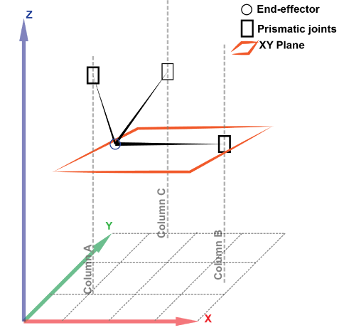
1. type 1 singularities: When and that is

The singularity occurs when one, two or even all 3 links are parallel to the XY or platform plane. A representation is given in Figure 7.

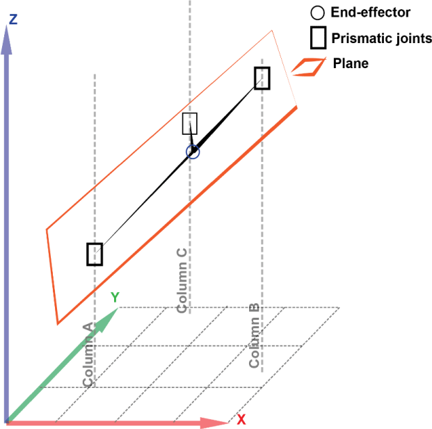
2. type 2 singularities: When and , that is

The singularity occurs when the 3 links are contained in the same plane. As shown in Figure 8.

3. type 3 singularities: When and the three links are parallel to the XY or platform plane. As depicted in Figure 9.

Results

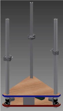
Once the study of the geometrical and kinematic aspects of the robot is done we proceeded to the conceptual design phase. During the conceptual design decision making we used the previously mentioned criteria of flexibility of design and modularity. An example of the aforementioned can be seen in Figures 7 and 8. Where the resulting links are mechanically jointed to the platform and the prismatic joints by means of spherical magnets. These magnetic joints works as a spherical joint and complies with the required 2 degrees of freedom required by the universal joint. Also, the link lengths can be modified in order to test other possible configurations. Regarding the modularity mentioned in section 3, the design of the prismatic actuators is done as an assembled modular unit. In this way a future project might use this element for a different robotic architecture.

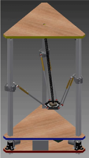
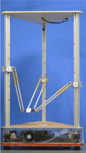
Following the criteria and kinematic modelling explained in sections 3 and 4 we arrive to a CAD prototype of the robot shown in Figure 9. After the manufacture and assembly of components according to the proposed design we arrived to the prototype depicted in Figure 10.

After construction and calibration by means of 3 end-stop sensors at the top of the prismatic joints, our prototype was ready for experimentation. In order to test the robot we defined a helix trajectory of centered in the center of the base, of radius 200mm and feed it to the open-source controller using Cartesian positions. While executing the trajectory of the helix, the joint trajectories were tracked as explained in section 3.

Joint tracking

Once the end-effector trajectories had been obtained and recorded in long exposure photographs, videos were made to obtain the trajectories of the prismatic joints and thus provide a basis for comparison. These trajectories were then processed by the direct kinematics in order to obtain an image similar to the corresponding photograph.

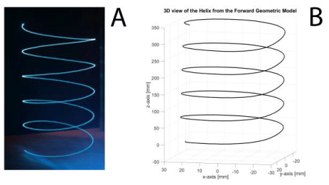
An example of this is given in the following Figure 11 where a visual comparison of the trajectory is obtained with a long time exposure photography with that obtained with the direct kinematics of the data measured from the prismatic joint tracking.

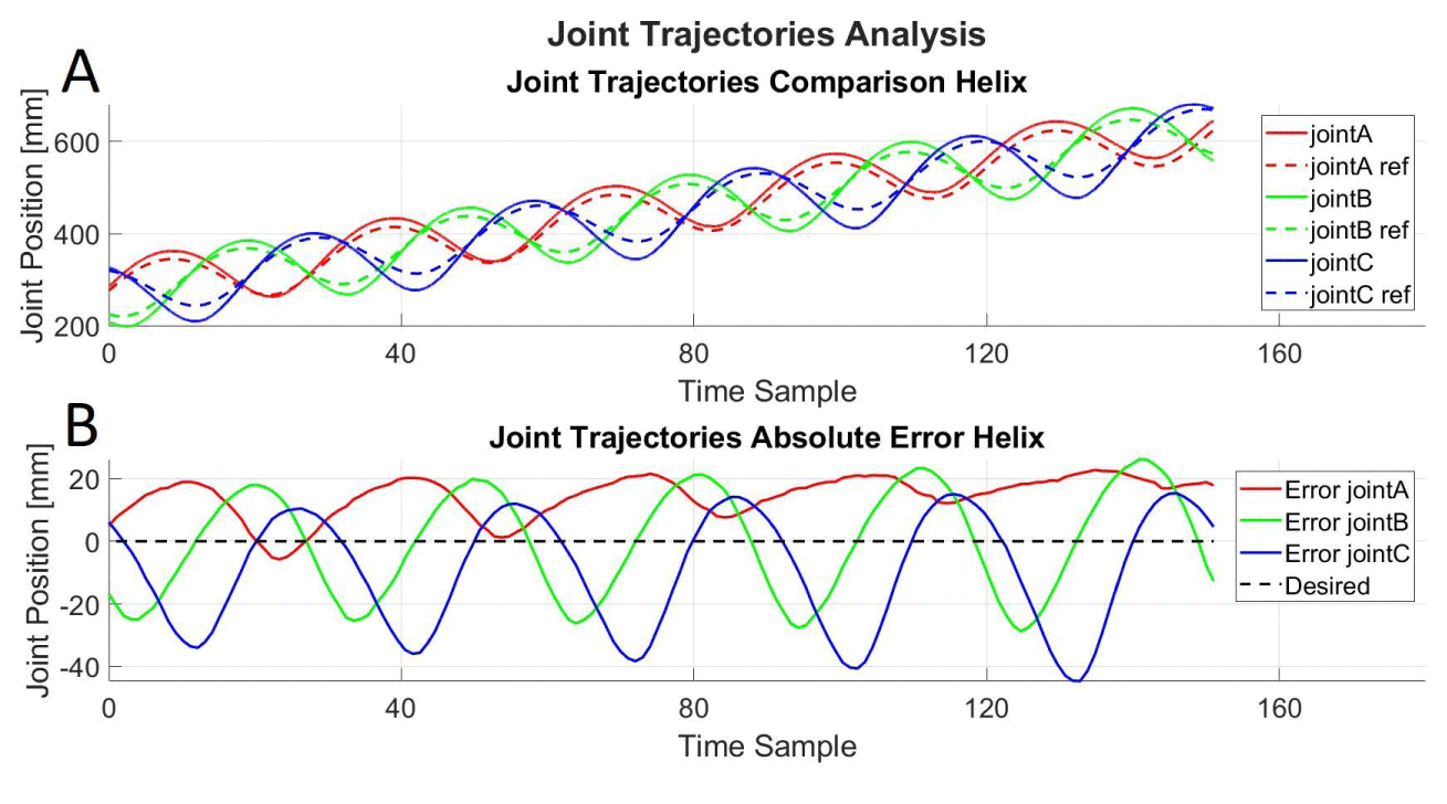
Afterwards with the obtained measures we were interested in continue to validate the kinematic model of the robot. With this in mind, we compared the reference helix trajectory with the measured data in the joint space of the robot. In this way arriving to the representation in Figure 2 where we plotted the reference and the measured joint trajectories and the absolute error. Additionally we were also interested in measure the correlation between the reference and measured joint values and we presented it in Table 1

At this point with all the presented results we proceeded to the discussion and conclusions of the work.

Discussion

For ease of the analysis of the obtained results we will first discuss the resulting design of the robot and then the kinematic aspects from the measurements made. With respect to the design of the robot we can say that the result is very approximate to the CAD as it can be seen from Figures 12,13. Some of the decisions, already remarked in sections 3 and 5, like the modularity and flexibility of design, for sure were very helpful for calibration and for solving issues derived from the construction of the prototype.

Nonetheless, because of the lack of access to stateof-the-art workshops, defects related to recycled components like the drives, manufacture and the short times of the project, the constructed prototype as it is, had some errors that later on are noticeable in the performance of the trajectories and will be discussed below.

With regards to the kinematic validation of the robot, in Figure 14 and 15 we can see that the result is visually quite similar and also correlated (Table 1). Helical trajectories allowed us to visualize a range of oscillatory movements of the prismatic joints whose mean value is shifted as the trajectory develops in the end effector. This type of trajectory is excellent for comparing the measured values with the reference values and for validating the kinematic model. But, when we go into the details the errors are quite significant for additive manufacturing applications and since we have a big working space the errors are not so noticeable in Figure 14. Nonetheless, a first detail is that the helix radius was set to be 20mm and in Figure 14B we can see distortion.

Afterwards, when analysing Figure 15B where one of the biggest errors is more than 40mm, it is clear that for achieving an accuracy around 0.5mm as obtained in [20] and a tolerance of ±0.2mm associated to produced parts using the Extrusion Thermal process, some improvements should be considered.

Among the actions that can be taken into account to reduce the errors, we consider two approaches, hardware, and software-wise. Within the mechanical details that can be improved, we consider that excentricity in the motors and pulleys and friction in the slider components are potential causes of errors. On the other hand, in the software part, we can improve the controllers by adding encoders so in case of loss of motor steps a closed loop action can put the robot back on track with the desired trajectory.

It is worth adding that even though the errors are considerable, the kinematic behavior of the joints with respect to the desired values are significantly correlated as displayed in Table 1. All of the prismatic joints of the robot present a high linear correlation between the reference and measured joint trajectories. This result enables us to say that, despite the errors, the kinematic model of the parallel kinematic robot proposed is validated.

Conclusion

In the present work, a robotic platform with parallel kinematic chains for Additive Manufacturing applications (3D printing) with a cylindrical workspace of 300mm in diameter by 300mm high was designed. The scope of our work covered the kinematic modeling approach to parallel robot design, presenting a design with flexible and modular characteristics that can be arranged to modify its own workspace and even shape new designs. Details going from the numerical simulation model of a 3 degree of freedom parallel robot up to the designed and construction were covered in this article. The preliminary results obtained from the real robot compared to the model by means of open source software for control and for measurement gave an insight on the state of the real platform and joint positions and enabled us to validate the kinematics of the mechanism. Establishing a methodology that can be used for designing this kind of robots.

This work promotes the development of future research works that combine the areas of design, manufacturing processes, automation, and robotics in countries in development such as Venezuela.

Finally, considerations were given regarding the assembly details that from the recycled components and difficulties related to the manufacturing the robot.

Future works

After investigating, understanding and modelling what is relevant to parallel kinematic robots for additive manufacturing applications the recommendations that were observed and distinguished, will be presented below.

Implement a closed-loop control strategy on the robot by means of a motor encoder, so we can be able to add accuracy to the tracking of the joint position. The precise tracking can allow us to know the exact position of the end-effector without the need to reset its position at the end-stop sensor, while at the same time improving the robot overall precision.

The modelling of the dynamic model will be useful since we want to exploit the speed of the robot. Earning awareness of the forces, accelerations and vibrations associated with the movements of the machine will enable us to achieve high performances. Future works will also include a deepest approach to the design aspects in order to propose novel solutions to this already developed robot architecture.

Finally, from its flexible and modular design, there is interest to continue the development of this robot in the field of reconfigurable robots and how can this be exploited to create a more dynamical robot optimizing the transmission of motion inside the workspace.

1. Kenton W (2021) Manufacturing. Investopedia.  Link: https://bit.ly/3x6u54W
2. Sarcar M, Rao K, Narayan K (2008) Computer aided design and manufacturing. PHI Learning.  Link: https://bit.ly/3iv3jz8
3. Thomas D, Gilbert S (2014) Costs and cost effectiveness of additive manufacturing. Link: https://bit.ly/3wkkcRn
4. Marinescu ID, Rowe B, Ling Y, Wobker HG (2015) Chapter 3 - abrasive processes. In ID Marinescu, TK Doi, E Uhlmann (Eds.), Handbook of ceramics grinding and polishing. William Andrew Publishing 67-132.  Link: https://bit.ly/353gsHW
5. Borunda L, Rodriguez Ladron de Guevara M, Pugliese G, Claramunt R, Mun˜oz M, et al. (2020) Componentes optimizados de fabricaci´on de aditivos = optimized additive manufacturing building components. Anales de Edificacion 6. Link: https://bit.ly/34Z4vTw
6. RepRap (2020) Reprap. Link: https://bit.ly/2SkP5Go
7. Merlet JP, Gosselin C (2008) Parallel mechanisms and robots. 269-285.  Link: https://bit.ly/3g4g81O
8. Schey J (2002) Procesos de manufactura. McGraw-Hill. Link: https://bit.ly/3x75Mnj
9. Kalpakjian S, Schmid S, Murrieta J (2014) Manufactura, ingenierıa y tecnologıa. Pearson Educacion. 1. Link: https://bit.ly/3gfbxss
10. Cotec (2011) Fabricaci´on aditiva. Documentos Cotec sobre oportunidades tecnologicas.
11. Singh S, Ramakrishna S, Singh R (2017) Material issues in additive manufacturing: A review. Journal of Manufacturing Processes 25: 185–200. Link: https://bit.ly/3ctP2Pc
12. Seward N, Bonev IA (2014) A new 6-dof parallel robot with simple kinematic model. 2014 IEEE International Conference on Robotics and Automation (ICRA) 4061–4066. Link: https://bit.ly/3gpseBH  
13. Gosselin C, Kong X, Foucault S, Bonev I (2004) A fully-decoupled 3-dof translational parallel mechanism. Parallel Kinematic Machines in Research and Practice 595–610. Link: https://bit.ly/3ix13Y6
14. Kong X, Gosselin C (2011) Forward displacement analysis of a quadratic 4-dof 3t1r parallel manipulator. The quadrupteron Meccanica 46: 147–154. Link: https://bit.ly/3wdEhZy
15. Kong X, Gosselin CM (2005) Type synthesis of 5-dof parallel manipulators based on screw theory. Journal of Robotic Systems 22: 535–547. Link: https://bit.ly/3ixXQaL
16. Oleksandr S (2016) 5-dof parallel robot. Link: https://bit.ly/2RCSwrH
17. Briones L, Antonio  J (2009) Disen˜o, an´alisis y construcci´on de un robot paralelo traslacional. Investopedia. Link: https://bit.ly/3iGBVOX 
18. Gogu G (2007) Structural synthesis of parallel robots. part 1: Methodology 149. Link: https://bit.ly/3iu8bES
19. Hodgins J (2012) Design, optimization, and prototyping of a three translational degree of freedom parallel robot. Link: https://bit.ly/2RBygqi
20. Song X, Pan Y, Chen Y (2015) Development of a low-cost parallel kinematic machine for multidirectional additive manufacturing. Journal of Manufacturing Science and Engineering 137: 021005. Link: https://bit.ly/3g6w2IR
21. Amigo D (2012) Diseno y construccion de una impresora 3d delta. Escola d’Enginyeria de Barcelona Est Grau en Enginyeria Mecanica.
22. Christian W, Brown D (2009) Tracker, video analysis and modeling tool.
23. Kutzbach K (1929) Mechanische leitungsverzweigung. ihre gesetze und anwendungen. Maschinenbau: derBetrieb/ Wirtschaftlicher Teil 8: 710-716.
24. Germain C, Caro S, Briot S, Wenger P (2013) Optimal Design of the IRSBot-2 Based on an Optimized Test Trajectory. ASME 2013 International Design Engineering Technical Conferences Computers and Information in Engineering Conference. Link: https://bit.ly/3503yud
25. Briot S, Bonev IA (2010) Pantopteron-4: A new 3t1r decoupled parallel manipulator for pick-and-place applications. Mechanism and Machine Theory 45: 707–721. Link: https://bit.ly/3iogr9g  
26. Gosselin C, Angeles J (1990) Singularity analysis of closed-loop kinematic chains. IEEE transactions on robotics and automation 6: 281–290. Link: https://bit.ly/3zgDKHQ

© 2021 Lahoud M, et al. This is an open-access article distributed under the terms of the Creative Commons Attribution License, which permits unrestricted use, distribution, and reproduction in any medium, provided the original author and source are credited.